FFT with Python
Warning
The mathematical concepts covered in this section are not addressed in a formal manner.
They are presented only as a reminder, and shortcuts have been intentionally taken to facilitate the understanding of these concepts.
Fourier Transform
The Fourier Transform is a mathematical operation that transforms a time-domain signal (a signal that varies over time) into a frequency-domain representation. It breaks down a complex signal into its constituent sinusoidal components, essentially showing how much of each frequency is present in the original signal.
Key Concepts
Time Domain vs. Frequency Domain
The Fourier Transform converts a time-domain signal into this frequency-domain representation.
Time Domain: Describes how a signal changes over time.
Frequency Domain: Describes how much of the signal lies within each given frequency band.
Sinusoids as Building Blocks
Any complex signal can be thought of as being made up of simpler sinusoidal waves (sines and cosines) of different frequencies, amplitudes, and phases.
The Fourier Transform identifies these components and tells you their frequencies and amplitudes.
Mathematical Definition
For a continuous-time signal \(f(t)\), the Fourier Transform \(F(\omega)\) is defined as:
Where:
\(F(\omega)\) is the frequency-domain representation of the signal.
\(\omega\) (omega) is the angular frequency (in radians per second).
\(f(t)\) is the original time-domain signal.
\(e^{-j\omega t}\) is a complex exponential function representing sinusoids.
For animated explanations, refer to this YouTube video from the 3Blue1Brown channel: https://www.youtube.com/watch?v=spUNpyF58BY
For a better mathematical approach, refer to this website: https://www.thefouriertransform.com/
Inverse Fourier Transform
The process can be reversed using the Inverse Fourier Transform to convert the frequency-domain representation back to the time domain:
Discrete Fourier Transform (DFT)
When working with digital signals (discrete samples), we use the Discrete Fourier Transform (DFT), which operates on discrete data points. The DFT is defined as:
Where:
\(X[k]\) is the frequency-domain representation of the signal.
\(x[n]\) is the time-domain signal sampled at \(N\) points.
\(N\) is the total number of samples.
\(k\) corresponds to the frequency index.
Fourier Transform Properties
The Fourier Transform has several important properties:
Linearity: The transform of a sum of signals is the sum of their transforms.
Time Shifting: Shifting a signal in time corresponds to a phase shift in the frequency domain.
Frequency Shifting: Shifting a signal in frequency corresponds to multiplying by a complex exponential in the time domain.
Convolution: Convolution in the time domain corresponds to multiplication in the frequency domain, and vice versa.
Sampled signal
The DFT, and by extension the FFT, operates on a finite set of samples. This transforms a finite time-domain signal into a finite frequency-domain representation.
Sampling frequency
The Sampling Rate (\(fs\)) or frequency is the number of samples taken per second from the continuous signal. It defines the upper limit of the frequencies that can be accurately captured.
Number of samples
The Number of Points (\(N\)) is the number of stored samples of the signal. If the FFT is computed over \(N\) points (i.e., if your time-domain signal has \(N\) samples), the result will contain \(N\) frequency bins.
Periodicity of the spectrum
When you perform a DFT on a sampled signal, the resulting frequency-domain representation is inherently periodic.
This means that the frequency spectrum repeats itself every \(fs\).
The result \(X[k]\) is periodic with period \(N\).
This periodicity means:
Example
Consider a simple sine wave:
When applying the Fourier Transform to this sine wave, the result is two spikes (delta function) in the frequency domain at the frequency \(-f\) and \(f\) of the sine wave, indicating that the sine wave consists of only one frequency component.
Fast Fourier Transform
The Fast Fourier Transform (FFT) is an algorithm that efficiently computes the Discrete Fourier Transform (DFT) of a sequence or its inverse (IDFT). The FFT is a critical tool in digital signal processing, image processing, and many other fields that involve the analysis of signals and data.
The direct computation of the DFT involves \(O(N^2)\) operations for \(N\) data points, which can be computationally expensive, especially for large \(N\). The FFT reduces this complexity to \(O(N \log N)\), making it much faster and more practical for real-world applications, especially when dealing with large datasets.
Mathematical Representation
The DFT of a sequence \(x[n]\) of length \(N\) is given by:
Where:
\(X[k]\) is the output of the DFT, representing the amplitude and phase of the frequency component at \(k\).
\(x[n]\) is the input sequence (time-domain signal).
\(e^{-j2\pi kn/N}\) represents the complex sinusoidal basis functions.
Output data of the FFT
When you compute the Fast Fourier Transform (FFT) of a signal, the output is a set of complex numbers that represent the frequency components of the signal. These numbers provide information about both the amplitude (magnitude) and the phase of each frequency component present in the signal.
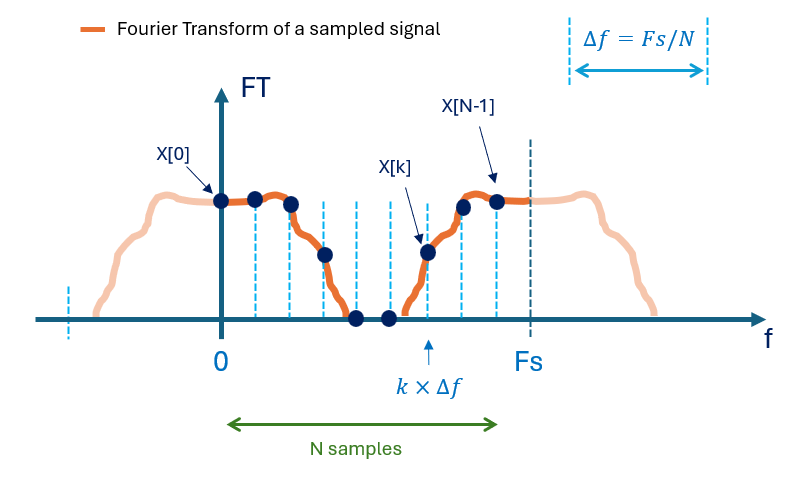
Fig. 8 Example of a discrete Fourier Transform output.
The output of the Fast Fourier Transform (FFT) process is a vector of the same size as the original input vector, consisting of \(N\) samples. Each sample in this output is spaced by \(\Delta{}f = \frac{f_S}{N}\), where \(f_S\) denotes the sampling frequency.
The \(k^{th}\) sample in the FFT output corresponds to the frequency component of the signal at the frequency \(k*\Delta{}f\).
Frequency axis
The frequency axis in the Fast Fourier Transform (FFT) represents the range of frequencies that are present in the signal being analyzed. Understanding how this axis is constructed and interpreted is crucial for analyzing the frequency content of a signal.
The FFT process partitions the frequency range from 0 Hz to :math:`f_S` into \(N\) equally spaced points. It is important to note that the frequency value :math:`f_S` itself is excluded from this interval due to the periodic nature of the Fourier transform applied to a sampled signal. Consequently, the frequency components are represented in the range \(\[0, f_s\[\), ensuring that the highest frequency is \(f_S - \Delta{}f\), where \(\Delta{}f = \frac{f_S}{N}\).
Frequency Resolution
The frequency difference between consecutive bins is given by:
This is the smallest frequency difference that the FFT can resolve.
Frequency bins
The FFT output is organized into “bins”, each corresponding to a specific frequency. The number of bins is equal to the number of samples \(N\) used in the FFT. Each bin represents a specific frequency, calculated as:
Where
\(f_k\) is the frequency corresponding to the \(k\)-th bin.
\(f_s\) is the sampling rate.
\(N\) is the number of samples or the size of the FFT.
Representation for physicians
Physicians and engineers often prefer to display the frequency range from negative to positive to provide a complete view of the signal’s frequency content.
This centered frequency spectrum allows for easier interpretation of certain phenomena, such as symmetry, phase shifts, and frequency modulation effects, which are crucial in many physical systems.
But, the standard FFT algorithm, when applied to a real-valued signal, typically outputs a frequency spectrum from 0 to \(fs\).
We assume that the frequency spectrum computed by a FFT on a sampled signal repeats itself every \(fs\) (the sampling frequency). For real signals, the Fourier Transform exhibits conjugate symmetry. This means that the positive and negative frequency components are mirror images of each other. So, the second half of the FFT output, corresponding to frequencies from \(\frac{fs}{2}\) to \(fs\), mirrors the first half because of the symmetry of real signals.
Ensure to respect the sampling theorem
It is very important to ensure that the Nyquist-Shannon sampling theorem is respected when using the Fast Fourier Transform (FFT).
Respecting the Nyquist-Shannon criterion when using FFT is crucial for:
Preventing aliasing and ensuring that the signal is accurately captured.
Obtaining a true and interpretable frequency-domain representation of the signal.
The Nyquist-Shannon sampling theorem states that for accurate representation and reconstruction of a continuous-time signal from its samples, the signal must be sampled at a rate that is at least twice the highest frequency present in the signal. This rate is known as the Nyquist rate.
Mathematically, if the highest frequency in a signal is \(f_{\text{max}}\), the sampling frequency \(f_s\) must satisfy:
Calculate the FFT of a signal
Calculating the Fast Fourier Transform (FFT) of a function in Python can be done using the numpy library.
Define the function
Note
This step is optional if your data is already stored in an appropriate object (an ndarray for example).
Let’s define a simple function, such as a sine wave, and create an array of sample points.
Note
The code of this example is in the \progs\numpy\numpy_fft.py file of the repository.
# Sampling parameters
sampling_rate = 1000 # Samples per second
T = 1.0 / sampling_rate # Sampling interval
N = 300 # Number of sample points
t = np.linspace(0.0, N*T, N, endpoint=False) # Time vector
# Define the function (e.g., sine wave with frequency 50 Hz)
frequency = 50 # Frequency in Hz
amplitude = 1.0 # Amplitude of the sine wave
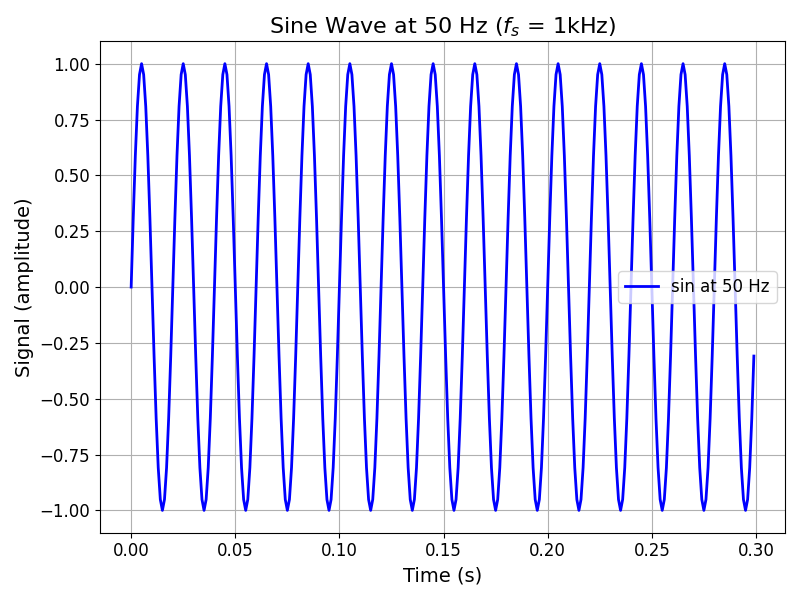
signal = amplitude * np.sin(2.0 * np.pi * frequency * t)
This example produces a sine signal at 50Hz shown in the following figure:
Compute the FFT
The FFT can be computed using numpy.fft.fft() method.
# Compute the FFT
fft_result = np.fft.fft(signal)

# Take the magnitude of the FFT result and normalize
fft_magnitude = np.abs(fft_result) / N
Construct Frequency Axis
Homemade Version
The goal is to create a vector representing the frequency axis, where the frequencies are given by this expression:
It’s possible to use the numpy.linspace() method.
xf = np.linspace(0, 1, N) * Fs
To change the frequency higher than \(f_s/2\) to the negative part of the spectrum, you can use this code:
condition = xf > Fs/2
xf[condition] = -(Fs - xf[condition])
And finally, to obtain a vector from \(-f_s/2\) to \(f_s/2\), it’s possible to use the numpy.fft.fftshift() method.
xf = np.fft.fftshift(xf)
Warning
If you want to display the FFT result using the latest version of xf, you also need to shift the FFT data to obtain a relevant graph.
fftfreq function
The frequency axis can be computed using numpy.fft.fftfreq() method.
# Compute the frequency axis
frequencies = np.fft.fftfreq(N, T)
This method requires the number of sample points (\(N\)) and the interval between two samples (or the sampling interval \(T_s = \frac{1}{f_s}\)).
With this two parameters, the frequency axis can be reconstructed.
Warning
The fftfreq() method gives a frequency axis range from negative to positive value, i.e. from \(-\frac{f_s}{2}\) to \(\frac{f_s}{2}\), but in a vector starting with the positive frequencies followed by the negative ones.
frequencies = [0, … N/2-1, -N/2… -1] * Fs
Display the FFT of a signal
Displaying the Fast Fourier Transform (FFT) of a function can be done matplotlib for visualization.
# Create the figure and axis
fig, ax = plt.subplots(figsize=(12, 8), dpi=100, nrows=2, ncols=1)

ax[0].plot(t, signal)
ax[0].set_title("Original Signal")
ax[0].set_xlabel("Time [s]")
ax[0].set_ylabel("Amplitude")
ax[0].grid(True)

ax[1].plot(np.fft.fftshift(frequencies), np.fft.fftshift(fft_magnitude))
ax[1].set_title("FFT of the Signal")
ax[1].set_xlabel("Frequency [Hz]")
ax[1].set_ylabel("Magnitude")
ax[1].grid(True)

plt.tight_layout()
plt.show()
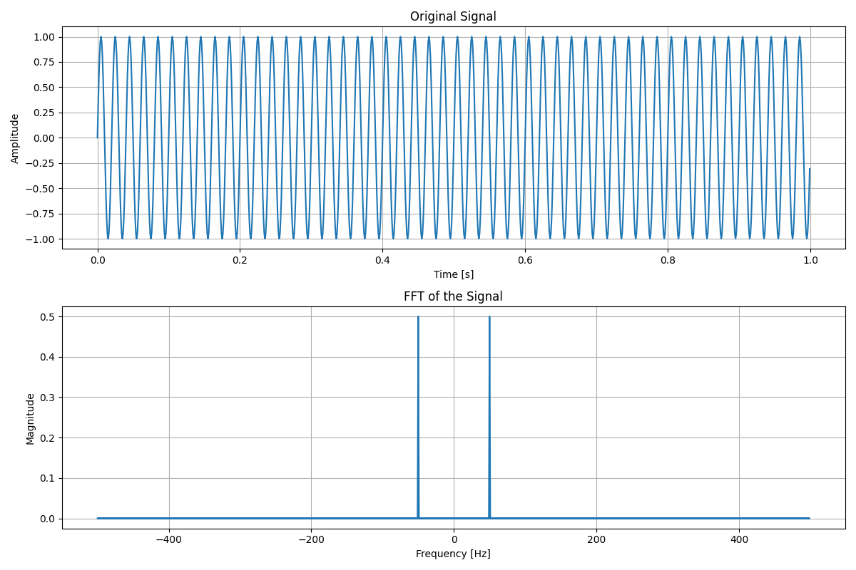
This example produces the following figure, showing the original signal (sine wave at 50Hz sampled at 1kHz) and its FFT: