Blur filtering with OpenCV
Blur on an image
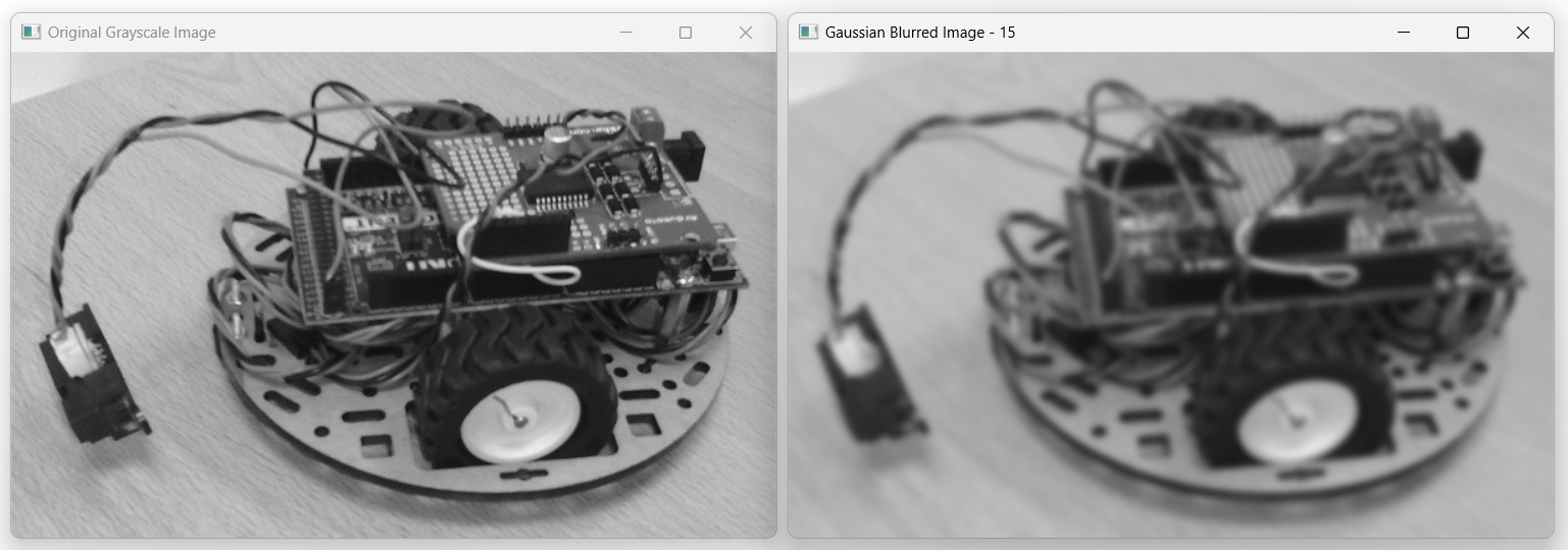
Blurring an image is a process in which the sharpness of the image is reduced, making edges and fine details less distinct. This is typically done by averaging the pixels within a certain neighborhood around each pixel in the image. The result is a softened image where details are less pronounced.

Fig. 12 Example of blurring of an image (Gaussian Blur - kernel of size 15).
There are different kinds of Blur:
Gaussian Blur: Applies a Gaussian function (a bell-shaped curve) to the pixels. It’s widely used due to its natural-looking blur effect.
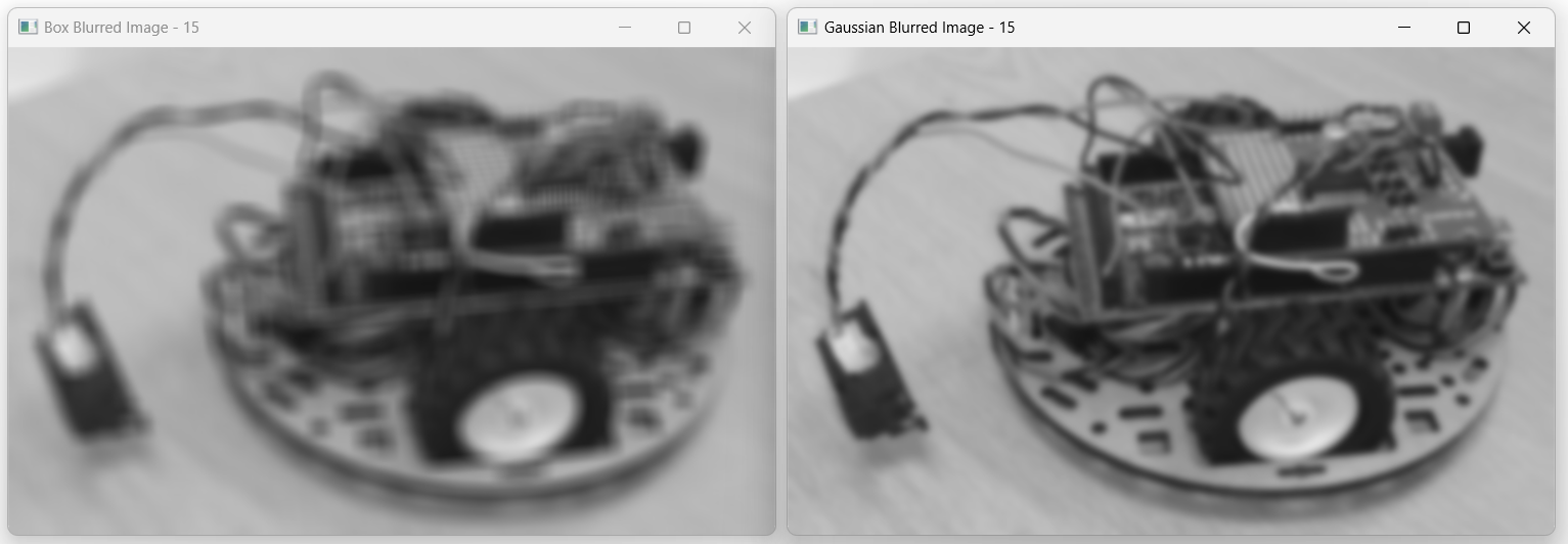
Box Blur (Averaging Blur): Averages the pixels within a square neighborhood. This type of blur is simpler but can introduce artifacts, such as “blockiness.”
Median Blur: Replaces each pixel’s value with the median value of the surrounding pixels. This type of blur is particularly good at removing noise while preserving edges.
Motion Blur: Simulates the effect of the camera or object moving during exposure, causing a directional blur.
The main applications of that kind of filter are: Noise Reduction, Image Preprocessing, Aesthetic Effects, Depth of Field Simulation, Data Privacy…
Note
The code of this example is in the \progs\Python\08_opencv_mean_filters\08_opencv_mean.py file of the repository.
Examples of images are stored in \_data\ directory of the repository.
Blur with OpenCV
Blur filters require a convolution kernel to process the image.
This kernel defines how the convolution process will modify each pixel in the image. It determines the type and extent of the effect (like blurring, sharpening, or edge detection) by specifying how neighboring pixels contribute to the output.
(see …)
In the case of blurring, the kernel is a square matrix whose size is determined by an odd integer.
kernel_size = (15, 15)
Gaussian blur
Gaussian Blur uses a kernel based on a Gaussian distribution, giving more importance to closer pixels and resulting in a smoother, more natural blur.
For example, a 3x3 kernel gives this resulting matrix:
And after normalizing:
To perform a gaussian blur filter on an image with OpenCV, you have to use the GaussianBlur function:
blurred_image_15_gauss = cv2.GaussianBlur(grayscale_image, kernel_size, 0)
Averaging blur (or Box)
Box Blur uses a uniform kernel where all neighboring pixels are averaged equally, resulting in a simpler but sometimes rougher blur.
For example, a 3x3 kernel gives this resulting normalized matrix:
To perform a averaging blur filter on an image with OpenCV, you have to use the blur function:
blurred_image_15_box = cv2.blur(grayscale_image, kernel_size)

Fig. 13 Comparison of a box blur filter (left) and a Gaussian blur filter (kernel of size 15).
Comparison between RGB and Grayscale images
We can compare the execution time of the blur process applied on the original RGB picture and on its grayscaled version by using this code:
import timeit
kernel_size = (15, 15)
# Blur on a grayscale image
def grayscale_process():
    blurred_image15g = cv2.GaussianBlur(grayscale_image, kernel_size, 0)
# Blur on a RGB image
def rgb_process():
    blurred_image15g = cv2.GaussianBlur(image, kernel_size, 0)

# Measure execution times
time_gray = timeit.timeit(grayscale_process, number=10)
time_rgb = timeit.timeit(rgb_process, number=10)

print(f"Execution time for Grayscale: {time_gray / 10:.6f} seconds")
print(f"Execution time for RGB: {time_rgb / 10:.6f} seconds")
On a specific computer, we obtained these results:
Execution time for Grayscale: 0.000267 seconds
Execution time for RGB: 0.000757 seconds
The RGB process is around 3 times slower than the grayscale process.